공부를 하는 입장이기 때문에, 내용에 오류가 있을 수 있습니다. 오류가 있다면 적극적으로 알려주시면 감사합니다!
1. Two Layer Network
학습하기 위한 2층 신경망을 구성하는 예제 코드이다. Neueral_network_learning.two_layer_net.py에서 확인할 수 있다.
import sys, os
# 내경로가 현재 폴더가 아닌 상위 폴더로 바꿈 # 부모 디렉터리의 파일을 가져올 수 있도록 설정
sys.path.append(os.path.dirname(os.path.abspath(os.path.dirname(__file__))))
import numpy as np
from Neueral_network_learning.numetical_gradient import numerical_gradient
from Neueral_network_learning.cross_entropy_error import  cross_entropy_error
from Neural_network.sigmoid import sigmoid
from Neural_network.softmax import softmax
import time

class TwoLayerNet:
    def __init__(self, input_size, hidden_size, output_size, weight_init_std=0.01):

        self.params = {}
        self.params['W1'] = weight_init_std * np.random.randn(input_size, hidden_size)
        self.params['b1'] = np.zeros(hidden_size)
        self.params['W2'] = weight_init_std * np.random.randn(hidden_size, output_size)
        self.params['b2'] = np.zeros(output_size)


    def predict(self, x):
        W1, W2 = self.params['W1'], self.params['W2']

        b1, b2 = self.params['b1'], self.params['b2']

        a1 = np.dot(x,W1) + b1
        z1 = sigmoid(a1)
        a2 = np.dot(z1, W2) + b2
        y = softmax(a2)

        return y

    def loss(self, x, t):
        y = self.predict(x)
        return cross_entropy_error(y,t)

    def accuracy(self, x, t):
        y = self.predict(x)
        y = np.argmax(y, axis=1)
        t = np.argmax(t, axis=1)

        acurracy = np.sum(y == t) / float(x.shape[0])
        return acurracy

    def numercial_gradient(self, x, t):
        loss_W = lambda W: self.loss(x, t)

        grads = {}
        grads['W1'] = numerical_gradient(loss_W, self.params['W1'])
        grads['b1'] = numerical_gradient(loss_W, self.params['b1'])
        grads['W2'] = numerical_gradient(loss_W, self.params['W2'])
        grads['b2'] = numerical_gradient(loss_W, self.params['b2'])

        return grads

if __name__=='__main__':
    net = TwoLayerNet(input_size = 784, hidden_size=100, output_size=10)
    print(net.params['W1'].shape)
    print(net.params['b1'].shape)
    print(net.params['W2'].shape)
    print(net.params['b2'].shape)

    x = np.random.rand(100, 784)
    t = net.predict(x)

    start_time = time.time()
    grads = net.numercial_gradient(x, t)
    end_time = time.time()

    print(f"Gradient calculation took {end_time - start_time:.2f} seconds")
    print(grads['W1'].shape)
    print(grads['b1'].shape)
    print(grads['W2'].shape)
    print(grads['b2'].shape)
def numerical_gradient(f, x):
    h = 1e-4 # 0.0001
    grad = np.zeros_like(x)

    it = np.nditer(x, flags=['multi_index'], op_flags=['readwrite'])
    while not it.finished:
        idx = it.multi_index
        tmp_val = x[idx]
        x[idx] = float(tmp_val) + h
        fxh1 = f(x) # f(x+h)

        x[idx] = tmp_val - h
        fxh2 = f(x) # f(x-h)
        grad[idx] = (fxh1 - fxh2) / (2*h)

        x[idx] = tmp_val # 값 복원
        it.iternext()

    return grad
self.numercial_gradient 함수 부분은 수치미분을 통해 계산한 기울기 값을 받는 함수이다. 수치 미분은 간단하게 말하면, 우리가 수학적으로 미분식을 구하는 것과 달리 수치적인 기울기 근사 값을 구하는 방식이다. (작은 변화(h)를 주고 그 변화를 통해 기울기를 근사 하는 방식, 더 자세한 것은 수치 해석을 살펴보자)
numercial_gradient 같은 경우는 함수 f와 함수의 편미분을 진행할 매개변수 x를 받는다. 따라서 이의 형태를 맞추기 위하여 인자 한 개를 받는 loss_W 함수를 람다 함수로 만든다.
예를 들어 grads['W1'] = numerical_gradient(loss_W, self.params['W1'])부분을 실행한다 해보면 numerical_gradient 속 매개 변수는 다음과 같다.
- 매개 변수 f : loss_W 함수는 W인자를 받지만 W를 사용하는 게 아닌 self.loss(x, t) 함수가 실행(즉, x와 t는 바뀌지 않는 고정 값)
- 매개 변수 x : self.param['W1']
while 문 3번째 줄을 살펴보면, 파라미터의 값이 바뀌게 되는 것을 확인할 수 있다.
이 부분이
x[idx] = float(tmp_val) + h
아래와 같이 저장된다
self.params['W1'][idx] = float(self.params['W1'][idx]) + h
그 후 함수를 실행하게 된다면 x와 t를 비롯해서 모든 매개변수는 그대로 있지만 W1 만 바뀐 상태로 loss_W 함수인 self.loss(x, t) 함수가 실행이 되게 된다.
fxh1 = f(x) # f(x+h)
아래와 같이 실행되겠지만 loss_W함수는 인자의 영향을 받지 않는다.
fxh1 = loss_W(self.params['W1'][idx])
이런 식으로 \(\frac{L(W1+h)-L(W1-h)}{2h}\)가 계산되어 \(\frac{\partial L}{\partial W1}\)이 계산된다.
마지막으로 self.params['W1']의 값을 원래로 돌리면 계산이 완료되고, 이를 W1 행렬 속 모든 값에 대하여 진행이 된다.
x[idx] = tmp_val # 값 복원
결과 값을 살펴보게 되면, W1, b1, W2, b2속 행렬의 모든 값에 미분을 했기 때문에 self.params의 크기와 grad속 크기가 같은 것을 알 수 있다.
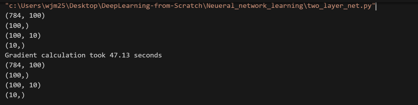
또한 수치미분을 하기 위해 많은 반복문을 선회하면서 47초라는 긴 시간이 걸린 것을 알 수 있다.
2. Train Two Layer Network
위에 코드를 바탕으로 실제로 학습을 진행하는 예제 코드이다. Neueral_network_learning.train_neural_net.py에서 확인할 수 있다.
import sys, os
# 내경로가 현재 폴더가 아닌 상위 폴더로 바꿈 # 부모 디렉터리의 파일을 가져올 수 있도록 설정
sys.path.append(os.path.dirname(os.path.abspath(os.path.dirname(__file__))))
import numpy as np
import matplotlib.pyplot as plt
from dataset.mnist import load_mnist
from Neueral_network_learning.two_layer_net import TwoLayerNet

(x_train, t_train), (x_test, t_test) = load_mnist(normalize=True, one_hot_label=True)

iter_num = 10000 # 반복 횟수
train_size = x_train.shape[0]
batch_size = 100 # 미니 배치 크기
learning_rate = 0.1

network = TwoLayerNet(input_size=784, hidden_size=50, output_size=10)

train_loss_list = []
train_acc_list = []
test_acc_list = []
# 1에폭당 반복 수
iter_per_epoch = max(train_size / batch_size, 1)

for i in range(iter_num):

    batch_mask = np.random.choice(train_size, batch_size)
    x_batch = x_train[batch_mask]
    t_batch = t_train[batch_mask]

    # 기울기 계산
    grad = network.numercial_gradient(x_batch, t_batch)

    # 매개변수 갱신
    for key in ('W1', 'b1', 'W2', 'b2'):
        network.params[key] -= learning_rate*grad[key]

    loss = network.loss(x_batch, t_batch)
    train_loss_list.append(loss)

    # 1에폭당 정확도 계산
    if i % iter_per_epoch == 0:
        train_acc = network.accuracy(x_train, t_train)
        test_acc = network.accuracy(x_test, t_test)
        train_acc_list.append(train_acc)
        test_acc_list.append(test_acc)
        print("train acc, test acc | " + str(train_acc) + ", " + str(test_acc))


plt.plot(range(len(train_loss_list)), train_loss_list)
plt.xlabel('Iteration')  # x축 레이블
plt.ylabel('Loss')       # y축 레이블
plt.title('Training Loss over Iterations')  # 제목
plt.grid(True)           # 그리드 추가
plt.show()
미니 배치를 구현하는 것은 굉장히 간단하다. 배치 사이즈만큼의 랜덤 행렬을 뽑아서 학습 데이터를 슬라이싱 하면 되는데 넘파이 배열의 경우 이를 쉽게 도와준다.
# train_size(1000)개 중에서 무작위로 batch_size(100)개의 인덱스 선택
batch_mask = np.random.choice(train_size, batch_size)
x_batch = x_train[batch_mask] # batch mask속 인덱스 만 선택해서 배열 생성
t_batch = t_train[batch_mask]
Epoch란 하나의 단위인데, 1 에폭은 학습에서 훈련 데이터를 모두 소진했을 때의 횟수에 해당한다. 예를 들어 해당 코드에서 데이터의 개수는 60000개이다. 따라서 1 에폭은 60000 / 100 = 600이 된다.
해당 코드는 학습이 잘 되고 있는지 판단하기 위해(훈련용 데이터에만 최적화되는지 확인하기 위해) 1에 폭당 학습 데이터와 테스트 데이터를 통해 정확도를 확인하는 부분이다.
    # 1에폭당 정확도 계산
    if i % iter_per_epoch == 0:
        train_acc = network.accuracy(x_train, t_train)
        test_acc = network.accuracy(x_test, t_test)
        train_acc_list.append(train_acc)
        test_acc_list.append(test_acc)
print("train acc, test acc | " + str(train_acc) + ", " + str(test_acc))'밑바닥부터 시작하는 딥러닝' 카테고리의 다른 글
| Backpropagation Example (0) | 2024.12.24 |
|---|---|
| Backpropagation (0) | 2024.12.24 |
| Neural Network Learning (0) | 2024.12.22 |
| Neural Network example (1) | 2024.12.20 |
| Neural Network (0) | 2024.12.19 |


